An introduction to queueing theory

We live surrounded by queues, we face them daily whether at the supermarket, driving on the way to work, or even consulting this post. If there is one thing that people especially dislike, it is waiting; there is nothing more frustrating for us than feeling our time slipping away while we wait in one.

Origins of queueing theory

To model these systems and to be able to study and optimize them (to make our lives more pleasant, of course) the Danish mathematician Agner Krarup Erlang published in 1909 the first approach to queueing theory.

With the growth of the telephone network at the time, it became necessary to know the most optimal way to scale it. The increase in the number of calls and users made it necessary to know what size should be assigned to the telephone switchboards. A switchboard that was too large, allowing a large number of connections, might be wasted in an area with few calls or with low traffic, and a small switchboard, not allowing many simultaneous connections, would always be saturated in an area with many calls or with high traffic.

Nowadays, systems such as traffic in a city, how many pumps are needed at a gas station, or simply the management of requests to a web server, are studied and optimized using the queueing theory base that Erlang initiated.

Structure of queueing systems

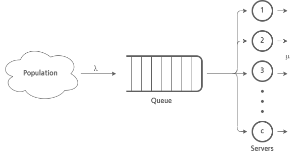
The following distinct components can be found in any queueing system:

• Input source or the population of customers that may come to request the service.
• The queues where customers wait to be served. There can be different types depending on the desired order of entry and exit.
• The stations where customers are served or servers.

Kendall’s notation

Kendall defined a notation to describe queueing models based on six characteristics (A/S/c/K/m/z) where:

• A specifies what the arrival process is like: whether inter-arrivals are i.i.d and Poissonian M, deterministic D, or follow some general distribution GI.
• S determines the service time distribution type. It is used the same notation as for arrivals.
• c is the number of servers.
• K is the system’s capacity or the number of places in the queue. If it is presumed to be infinity, it will be blank.
• N is the population size. If the population is presumed to be infinity, it will be also blank.
• D determines the queue’s discipline, or how priority is distributed among arriving customers. Whether it is a FIFO, LIFO, SIRO… If it is a FIFO queue it is not necessary to indicate it.

For example, the notation that would be used for a system with a Poissonian arrival and service rate, a single server, infinite capacity, and population, and a FIFO queue would be M/M/1.

With this, we could conclude this small approach to queueing theory. These systems are present in any area of our life. Without a doubt, getting to know them is exciting, don’t you think so?